The following is an explanation of how RetNet works. RetNet is a proposed modification / replacement to the Transformer architecture.
The explanation is aimed at someone who has a pretty ok idea of how Transformers and self-attention work -- for someone who has understood something like this and maybe written out a toy implementation of self-attention themselves. If you don't know what a residual connection, a MLP, or what self-attention are, you should not bother reading this.
I'm going to elide some details that would be necessary for an actual implementation -- i.e., most of my sample code will explain how a single-headed version of RetNet works, even though RetNet itself is multi-headed.
Why Care?
Why should you care what RetNet is?
Well, it aims to be an improvement to the Transformer -- to multi-head self-attention specifically, which it replaces with "multi-scale retention".
(I wish they hadn't renamed "multi-head" with "multi-scale" -- they're very nearly the same thing.)
Specifically, retention has three different modes of operation, which can be chosen as appropriate at training or inference times -- you use the same weights for each. These modes are as follows:
-
Parallel Mode: In this mode, GPU memory use increases with the square of sequence length, just like with attention. You can also do parallel training on a GPU, just like with attention. So -- this is basically attention, with some changes to allow you to switch it to the other two modes.
-
Recurrent Mode: This mode lets you incrementally a new token with constant O(1) memory and O(1) compute cost. This means that inference is much faster than inference with self-attention, because you don't slow down as the sequence gets longer.
- Recurrent Chunkwise Mode: This is kind of a cross between 1 and 2. During training, this lets you split training against a sequence of length 10,000 into 20 sequences of length 500. Total memory use is then (somewhat) as if you were only ever training against a sequence length 500, even though parallelization is decreased.
These are all interesting modes to have.
But RetNet is not the only model out there which claims to be able to train in parallel mode and do inference in recurrent mode -- RWKV can also do this.
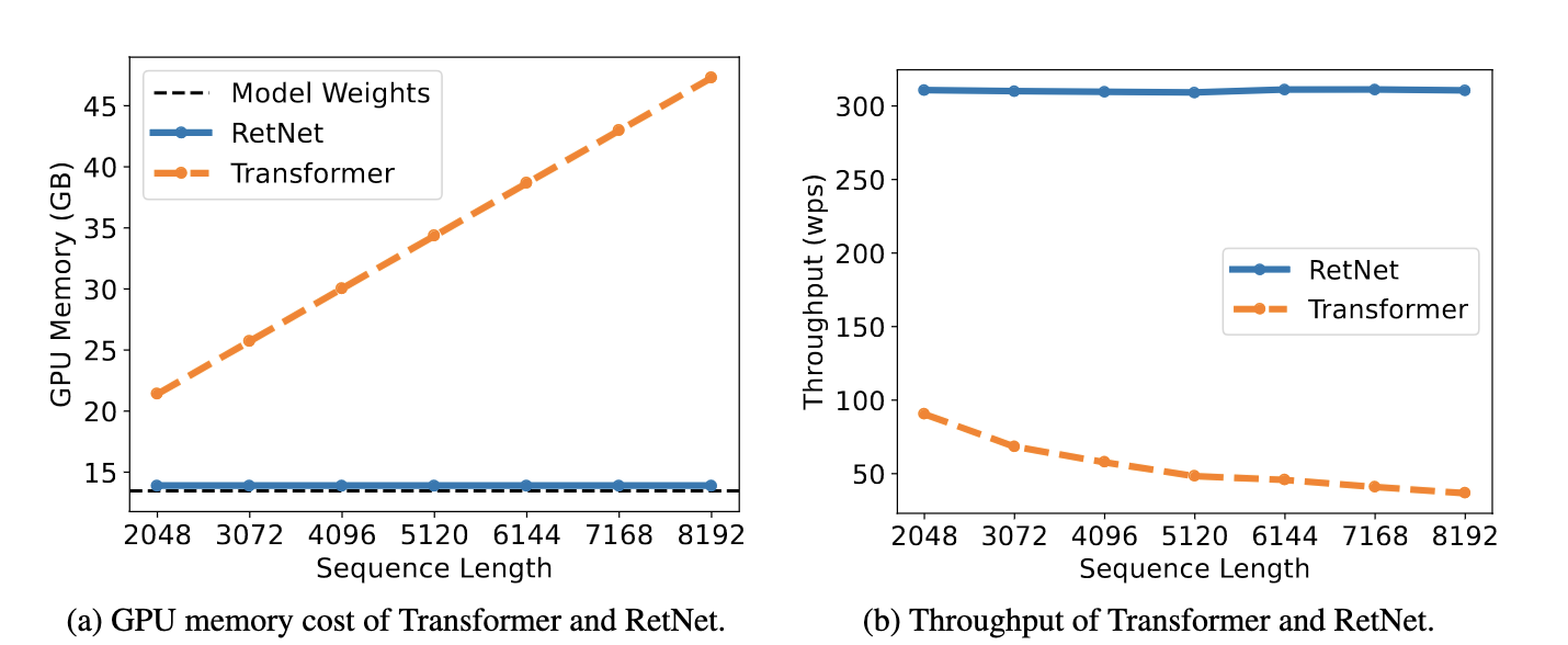
It does claim, however, that it maintains and even improves upon the performance of a transformer in a way no other model does. I'm somewhat skeptical of this -- although it's performance does look good. It actually claims to scale better than a transformer, which would be a huge deal if true.
Ok. So how does it work?
The Basics
Retention is best conceived of as a modification to attention.
The standard self-attention operation is something like softmax((Q(K^T)/sqrt(dim))V. (This leaves out causal masks for now).
Let's drop the softmax. That will cause problems -- but it will let us shuffle around parenthesis, which will open up opportunities for incremental calculation.
So for now, let's imagine that transformers just use this: (Q(K^T))V.
Now we can move the parentheses around, because (AB)C = A(BC) for matrices.
(Q(K^T))V = Q((K^T)V)
So the following two pieces of PyTorch code are equivalent:
import torch as t
import torch.nn as nn
import torch.nn.functional as F

T = 6 # length
D = 4 # dimension

X = t.randn(T, D)
Qw = t.randn(D, D)
Kw = t.randn(D, D)
Vw = t.randn(D, D)

# X = [t,dim] input, of length `t` with `dim` dimensions
# Qw, Kw, Vw = linear transform matrices for query, key, and values
#
def from_attention(X, Qw, Kw, Vw):
  Q = (X @ Qw)      # [t,dim] @ [dim, dim] == [t, dim]
  K = (X @ Kw)      # same
  V = (X @ Vw)      # same

  att = Q @ K.T     # [t,dim] @ [dim, t]   == [t, t]
  return att @ V    # [t,  t] @ [t, dim]   == [t, dim]

def from_retention(X, Qw, Kw, Vw):
  Q = (X @ Qw)      # [t,dim] @ [dim, dim] == [t, dim]
  K = (X @ Kw)      # same
  V = (X @ Vw)      # same
  Kv = K.T @ V      # [dim, t] * [t, dim] == [dim, dim]
  return Q @ Kv

# returns true everywhere
from_attention(X, Qw, Kw, Vw) == from_retention(X, Qw, Kw, Vw)
On its own, of course, this gets us precisely nothing so far -- we ge the same answer via an intermediary Kv matrix with [dim,dim] dimensions rather than an intermediary att matrix with [T, T] dimensions -- but let's see where we can go with it.
Unimportant Sidenote: One thing that's a little painful about this formulation is that in attention, the [T, T] matrix has an intuitive understanding -- it's how much each vector "is influenced by" to vectors near it.
So, for attention, high values of attention at the Nth row and Mth column mean that the Nth element in the sequence is influenced a lot by the Mth element in the sequence. (And this is, of course, why we have to mask out elements for causal transformers, so the 2nd element cannot be influenced by the 5th. More on that later.)
But... what is the natural interpretation of the [Dim, Dim] matrix? There isn't really one. It's going to be the "state" that we build up over the course of iteration in the non-parallel mode, but that's it.
An important thing about this Kv matrix is that is additive over the time element. That is, imagine if you make a [Dim, Dim] matrix by multiplying K^T with V, where K and V both are [32 x 256] matrices -- that is, they represent a sequence of length 32 and with dimension 256.
You can can get precisely the same matrix by taking each of the 32 [1 x 256] matrices from K and V, multiplying K^T by V for each, and getting 32 matrices with dimension of [256 x 256], and then adding them together.
This will open the way for incremental computation.
Building Intuition for Incremental Calculation
Note that you can calculate the [Dim, Dim] matrix for simply the first element in the sequence. Sadly, this does not equal the full result anywhere:
def from_retention_first_row(X, Qw, Kw, Vw):
  X = X[:1,:]      # CHANGE -- set x to be just the first row
  Q = (X @ Qw)      # [t,dim] @ [dim, dim] == [t, dim]
  K = (X @ Kw)      # same
  V = (X @ Vw)      # same
  Kv = K.T @ V      # [dim, t] * [t, dim] == [dim, dim]
  return Q @ Kv

# Doesn't match the full attention results anywhere,
# just returns a tensor full of "false"
from_attention(X, Qw, Kw, Vw) == from_retention_first_row(X, Qw, Kw, Vw)
Ok -- but what if we change attention to be a little more realistic?
Let's make a causal attention mask and add it to our attention implementation.
mask = t.tril(t.ones(6,6))
#tensor([[1., 0., 0., 0., 0., 0.],
#        [1., 1., 0., 0., 0., 0.],
#        [1., 1., 1., 0., 0., 0.],
#        [1., 1., 1., 1., 0., 0.],
#        [1., 1., 1., 1., 1., 0.],
#        [1., 1., 1., 1., 1., 1.]])

def from_attention_masked(X, Qw, Kw, Vw):
  T = X.shape[0]
  Q = (X @ Qw)      # [t,dim] @ [dim, dim] == [t, dim]
  K = (X @ Kw)      # same
  V = (X @ Vw)      # same
  mask = t.tril(t.ones(T, T))
  att = (Q @ K.T) * mask        # t x t
  v = (X @ Vw)                  # t x dim
  return att @ v

from_attention_masked(X, Qw, Kw, Vw) == from_retention_first_row(X, Qw, Kw, Vw)
# returns
# tensor([[ True,  True,  True,  True],
#        [False, False, False, False],
#        [False, False, False, False],
#        [False, False, False, False],
#        [False, False, False, False],
#        [False, False, False, False]])
Ok, so now our retention using just the first row of the data actually matches the masked attention for the first row, if the attention is masked. Why?
Let's work through algebraically why it comes to the same thing.
If you don't give a shit about this, and just want to see the code, skip to the next header -- I'm sympathetic to that point of view.
First, we know each operation -- attention and retention -- just uses data from the first row of X to calculate the first row of the output.
We know for attention, because the scalar at the [0,0] point of the attention matrix is simply the dot product of the first row of Q and the first row of K. The mask then means all the values other than the first row of V are zerod out, so the value output is simply the first row of V scaled by the dot product of Q and K.
And we know for retention, well, because we filter down to the first row of X at the start in the code for it.
Granted that they use the same data, though, why do the operations come to the same values?
For attention:
Well, attention gives us the dot product of the first row of Q and K times the first row of V. So the value here is (Q_1·K_1)*V_1, if *_1 means the first row of the matrix in question.
Let's work it out algebraically. The dot product of Q_1 and K_1 is q1 * k1 + q2 * k2 + q3 * k3.... We can multiply this by [v1, v2, v3...] to get the final value:
(q1 * k1 + ... + qn * kn) * v1,
(q1 * k1 + ... + qn * kn) * v2,
...
(q1 * k1 + ... + qn * kn) * vn
If you wanted to indice the values by the row and column, this is the sum of q1n * k1n over n times [v11, v12, ... v1n].
For retention:
The operation K_1^T @ V_1 creates a [dim, dim] matrix, because we're multiplying a [dim, 1] matrix by a [1, dim] matrix. In the [dim, dim] matrix, each entry is the result of multiplying a single value in K by a single value in V:
k1 * v1   |   k1 * v2   |   k1 * v3
-----------------------------------
k2 * v1   |   k2 * v2   |   k2 * v3
-----------------------------------
k3 * v1   |   k3 * v2   |   k3 * v3
Let's call this the Kv matrix, which is what the attention paper uses as shorthand for it. The Q_1, matrix is single-row [1, 3] matrix, so Q_1 @ Kv will multiply each column of the [dim, dim] Kv matrix by the single row of the Q_1 matrix by the definition of matrix multiplication. This gives us:
(k1 * v1) * q1 + (k2 * v1) * q2 + .... + (kn * v1) * qn, <-- one column of Kv * Q_1
(k1 * v2) * q1 + (k2 * v2) * q2 + .... + (kn * v2) * qn, <-- next column
...
(k1 * vn) * q1 + (k2 * vn) * q2 + .... + (kn * vn) * qn
Each row n only has the single vn element in it. That is, the first row has v1 in every multiplication, the second row has v2, and so on. So we can factor out the vn from each row:
(k1 * q1 + k2 * q2 + ... kn * qn) * v1,
(k1 * q1 + k2 * q2 + ... kn * qn) * v2,
(k1 * q1 + k2 * q2 + ... kn * qn) * v3,
...
Which is exactly the same as the result that we have from attention.
Incremental Retention
Ok, but who gives a shit about just calculating the first row of attention? We want the entire thing!
Well, if we loop over the time element, we can incrementally build up the Kv matrix necessary for each row.
def from_retention_incremental(X, Qw, Kw, Vw):

  # IMPORTANT CHANGE HERE ----
  result = []
  Kv = t.zeros(D,D)
  # --------------------------

  for i in range(T):
    Xt = X[i:i+1]      # stands for X at time t
    Q = (Xt @ Qw)      # [1,dim] @ [dim, dim] == [1, dim]
    K = (Xt @ Kw)      # same
    V = (Xt @ Vw)      # same

    # IMPORTANT CHANGE HERE -----
    Kv = Kv + K.T @ V  # D x D
    result.append(Q @ Kv)
    # ---------------------------

  return t.concat(result, dim=0)

from_attention_masked(X, Qw, Kw, Vw) == from_retention_incremental(X, Qw, Kw, Vw)
# tensor([[True, True, True, True],
#        [True, True, True, True],
#        [True, True, True, True],
#        [True, True, True, True],
#        [True, True, True, True],
#        [True, True, True, True]])
Note that here, we build up the Kv tensor by adding K.T @ V to it after every loop over X.
I originally worked out an algebraic expansion for the above, but let's honest no one is going to read it.
Chunkwise Code
This isn't everything we want, though. We still lack something between the incremental method and the parallel method.
Specifically, this would let us use our GPUs to do training in parallel (like attention) but would let us break up that parallel training into chunks, so that if we wanted to train over 10k tokens, the entire 10k x 10k attention map never had to be loaded into memory at once. Instead, we could break up the process into 20 500-token chunks and train with them.
We an do this with the chunkwise attention.
Note, again, that each of these different ways are mathematically equivalent -- you can use the same weights for any of them.
def from_retention_chunkwise(X, Qw, Kw, Vw, steps):

  lgt, dim = X.shape[0], X.shape[1]
  chunk_sz = lgt // steps
  mask = t.tril(t.ones(chunk_sz, chunk_sz))

  result = []
  past_kv = t.zeros(D, D)

  for i in range(steps):

    # Pull out a chunk from the input
    Xt = X[i * chunk_sz:(i+1) * chunk_sz,:]

    # Get QKV over the chunk
    Q, K, V = (Xt @ Qw), (Xt @ Kw), (Xt @ Vw)

    # standard attention over the chunk is how
    # we calculate values for it -- this is as if
    # we simply used attention
    att = (Q @ K.T) * mask
    inner_ret = att @ V

    # then we use 'past_kv' to calculate
    # values from the past
    past_ret = Q @ past_kv

    # output is the 'inner retention' -- the attention
    # plus the past retention
    result.append(inner_ret + past_ret)

    past_kv = past_kv + K.T @ V

  return t.concat(result, dim=0)

# return true everywhere
from_attention_masked(X, Qw, Kw, Vw) == from_retention_chunkwise(X, Qw, Kw, Vw, 3)
The above implements retention without any position encoding or time decay. So lets add some time decay, like AliBi. AliBi, or attention with linear biases, down-weights the attention for items further in the past. (The RetNet paper also uses xPos, a relative positional encoding, but I'm not going to get to that.)
It's easy to add add an AliBi-like decay to the causal mask. Note than in what follows here, we're combining the causal mask and the decay mask into one thing.
t_count = t.arange(0, T)
decay_mask = 0.5 ** (t_count.reshape(T, 1) - t_count.reshape(1, T))

# tensor([[1.0000e+00, 2.0000e+00, 4.0000e+00, 8.0000e+00, 1.6000e+01, 3.2000e+01],
#        [5.0000e-01, 1.0000e+00, 2.0000e+00, 4.0000e+00, 8.0000e+00, 1.6000e+01],
#        [2.5000e-01, 5.0000e-01, 1.0000e+00, 2.0000e+00, 4.0000e+00, 8.0000e+00],
#        [1.2500e-01, 2.5000e-01, 5.0000e-01, 1.0000e+00, 2.0000e+00, 4.0000e+00],
#        [6.2500e-02, 1.2500e-01, 2.5000e-01, 5.0000e-01, 1.0000e+00, 2.0000e+00],
#        [3.1250e-02, 6.2500e-02, 1.2500e-01, 2.5000e-01, 5.0000e-01, 1.0000e+00]])

decay_mask = t.tril(decay_mask)

#tensor([[1.0000, 0.0000, 0.0000, 0.0000, 0.0000, 0.0000],
#        [0.5000, 1.0000, 0.0000, 0.0000, 0.0000, 0.0000],
#        [0.2500, 0.5000, 1.0000, 0.0000, 0.0000, 0.0000],
#        [0.1250, 0.2500, 0.5000, 1.0000, 0.0000, 0.0000],
#        [0.0625, 0.1250, 0.2500, 0.5000, 1.0000, 0.0000],
#        [0.0312, 0.0625, 0.1250, 0.2500, 0.5000, 1.0000]])

def make_decay_mask(lngt, decay_factor):
  cnt = t.arange(0, lngt)
  zero_diagonal = cnt.reshape(lngt, 1) - cnt.reshape(1, lngt)
  decay_mask = decay_factor ** zero_diagonal
  return t.tril(decay_mask)

def from_attention_masked_decayed(X, Qw, Kw, Vw):
  decay_mask = make_decay_mask(X.shape[0], 0.9)
  att = (X @ Qw) @ (X @ Kw).T
  att = att * decay_mask
  v = (X @ Vw)
  return att @ v
And now for incremental retention, where the code is quite natural:
def from_retention_incremental_decayed(X, Qw, Kw, Vw):

  result = []
  decay_factor = 0.9
  Kv = t.zeros(D,D)

  for i in range(T):
    X_t = X[i:i+1]      # 1 X D
    Xq = (X_t @ Qw)     # 1 x D
    Kv_tmp = ((X_t @ Kw).T @ (X_t @ Vw))

    # Notice the change here is the only one
    # that needs to be made
    Kv = Kv * decay_factor + Kv_tmp  # D x D
    result.append(Xq @ Kv)

  return t.concat(result, dim=0)
Chunkwise Code With Incremental Decay
def from_retention_incremental_decayed_chunkwise(X, Qw, Kw, Vw, steps):

  # How many chunks to use
  decay_factor = 0.9
  lngt, dim = X.shape[0], X.shape[1]
  chunk_size = lngt // steps

  # [chunk_size x chunk_size]
  decay_mask = make_decay_mask(chunk_size, decay_factor)

  result = []
  past_kv = t.zeros(D, D)

  for i in range(steps):
    Xt = X[i * chunk_size:(i+1) * chunk_size,:]

    # All of these are [chunk_size, dim]
    Q = (Xt @ Qw)
    K = (Xt @ Kw)
    V = (Xt @ Vw)

    # standard attention pays attention to the
    # chunk almost as if it were simply a transformer
    # without the softmax

    # att: [chunk_sz x chunk_sz]
    att = Q @ K.T
    att = att * decay_mask

    # inner_at: [chunk_sz, dim]
    inner_att = att @ V

    # the recurrent part manages to add values
    # to the transformer-esque inner part

    # decay here needs to take into account how
    # the FURTHER UP a given element is, the more
    # the saved values need to decay.  So we're going
    # to be multiplying results by an array scaling from
    # [df ** 0 == 0, df, df ** 2 ... ] and so on.
    dec = (decay_factor ** t.arange(0, chunk_size, 1)).reshape(-1, 1)

    # Q:[T,D] Kv: [D,D] --> T,D
    cross_att = (Q @ past_kv) * dec

    # the actual results, we then get by
    # adding the inner attention + the cross
    # attention
    result.append(inner_att + cross_att)

    # elements CLOSER TO FRONT of the chunk are further
    # in the past, so we need to discount them more

    # so we multiply everything by something like
    # [df ** n, df ** (n - 1), ... , df ** 1]
    dec = (decay_factor ** t.arange(chunk_size, 0, -1)).reshape(-1, 1)

    past_kv_new = K.T @ (V * dec)
    past_kv_decayed = past_kv * (decay_factor ** chunk_size)
    past_kv = past_kv_decayed + past_kv_new


  return t.concat(result, dim=0)
Conclusion
I've left out a lot from my examples here. Specifically:
-
As attention is normally divided into several heads, so also is retention. The retention paper specifically refers to "multi-scale retention," because each head has a different time decay factor, but this is needless terminological innovation -- it just has multi-head attention like a transformer.
-
The output of each retention block is also put through a learned gating function. The learned gating function has as many parameters as the value projection -- so retention has more parameters per-layer than self-attention.
-
The output is also normalized with GroupNorm.
-
A relative positional encoding, xPos is also added to the data. (Although BlinkDL reports in the RWKV discord that the code works fine without it, so maybe this is unnecessary.)
I don't know if RetNet will take over.
I do think that -- given that inference costs for LLMs now dominate training costs -- we're going to see some kind of model that permits constant-memory inference take over. Between RetNet, RWKV, and so on, the potential gains seem enormous. Even if it takes 2x as much compute to train such a model to the same point, the ~10x or more decrease in inference costs makes such methods obvious choices.